Example 09: Tidal oscilation

Purpose

To calculate the open channel flow with a tidal oscilation at a boundary. In this example an open channel with dowsntream and upstream boundaries with constant discharge at upstream and oscilating water surface at downstream will be simulated. For simplicity only water is simulated and can add density flow if needed.

Creation of calculation grid and setting initial conditions

As explained in the other examples and the introduction, create the grid using, [Grid], [Select Algorithm to Create Grid] and then select [Grid Generator for Nays3DV]. Then the grid creation window will appear.

In grid creation window, give channel shape parameters as shown in Figure 133.

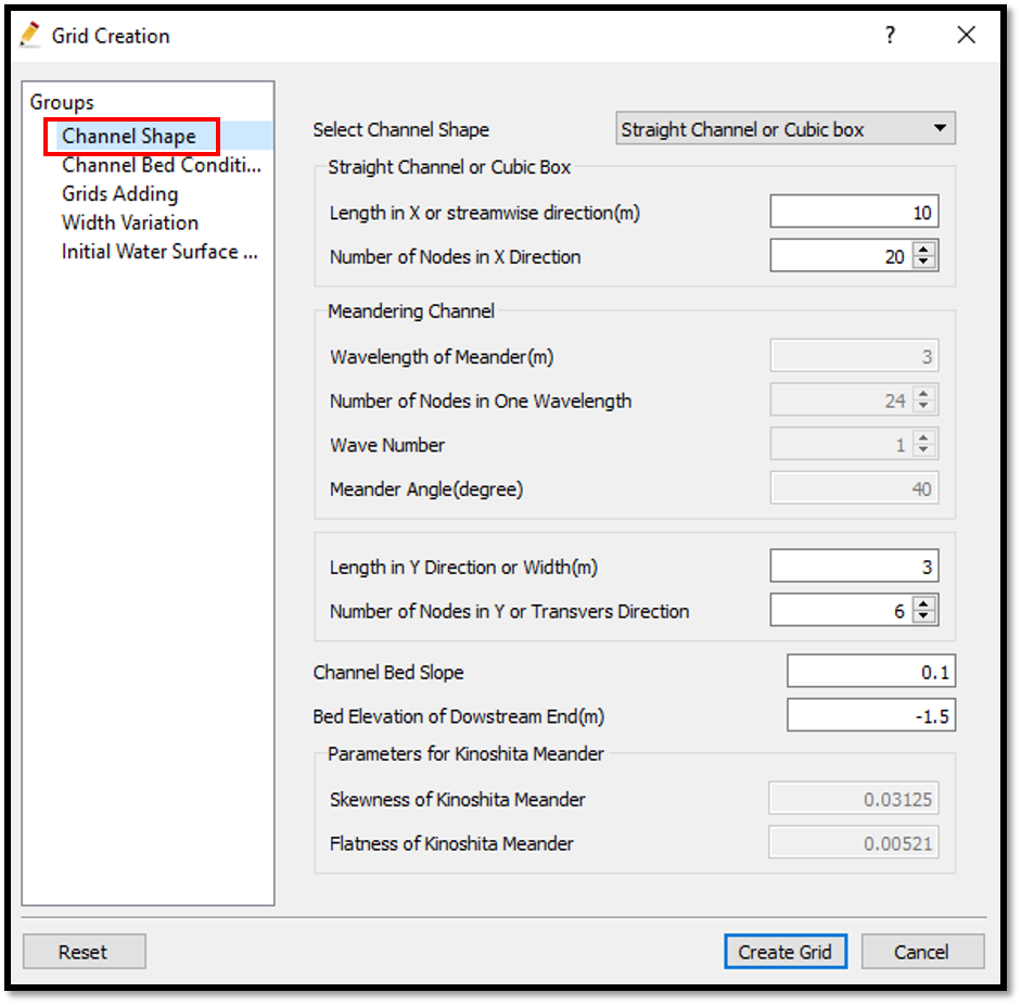
Figure 133 : Grid creation : Computational Domain

Then we can give Channel bed condition. As here we use the default condition flat(no bar) no modifications are needed.

If new grids are added or width is varied it is possible to set them. As in this example no grids added and no width variations, no modifications are needed in them.

Initial water surface profile tab is used to give downstream depth, water surface slope and initial water surface purtavation. It can be seen as shown in Figure 134 and click on [Create Grid]. Here the bed is given as a sloped bed varying linearly in x direction.

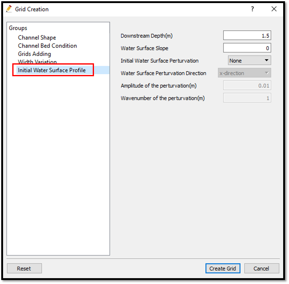
Figure 134 : Grid creation : Bed elevation and Depth

Then the grid is created and a confirmation message box will appear asking to map the geographic data as shown in Figure 135 and click on [Yes].

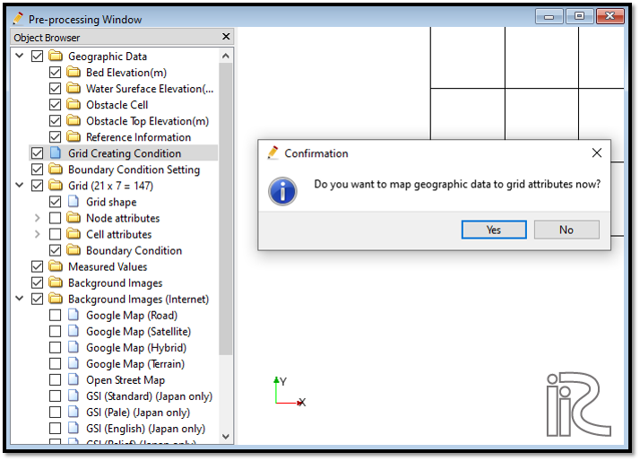
Figure 135 : Grid creation : Mapping geographic data to the grid

This will map the geographic data to the grid and the mapped grid can be seen as shown in Figure 136.

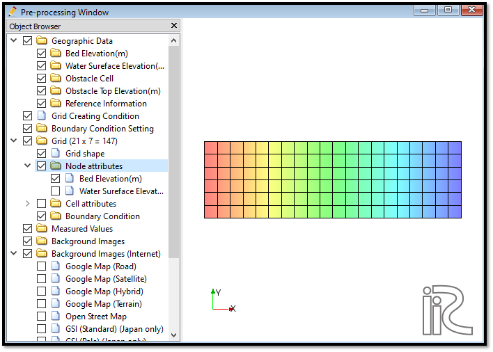
Figure 136 : Grid creation : Mapping geographic data to the grid

Now save the project with [File] [Save project as .ipro].

Setting the calculation conditions and simulation

Set the calculation conditions with [Calculation Condition], [Setting].

Calculation condition window will open.

Set computational parameters as shown in Figure 137.

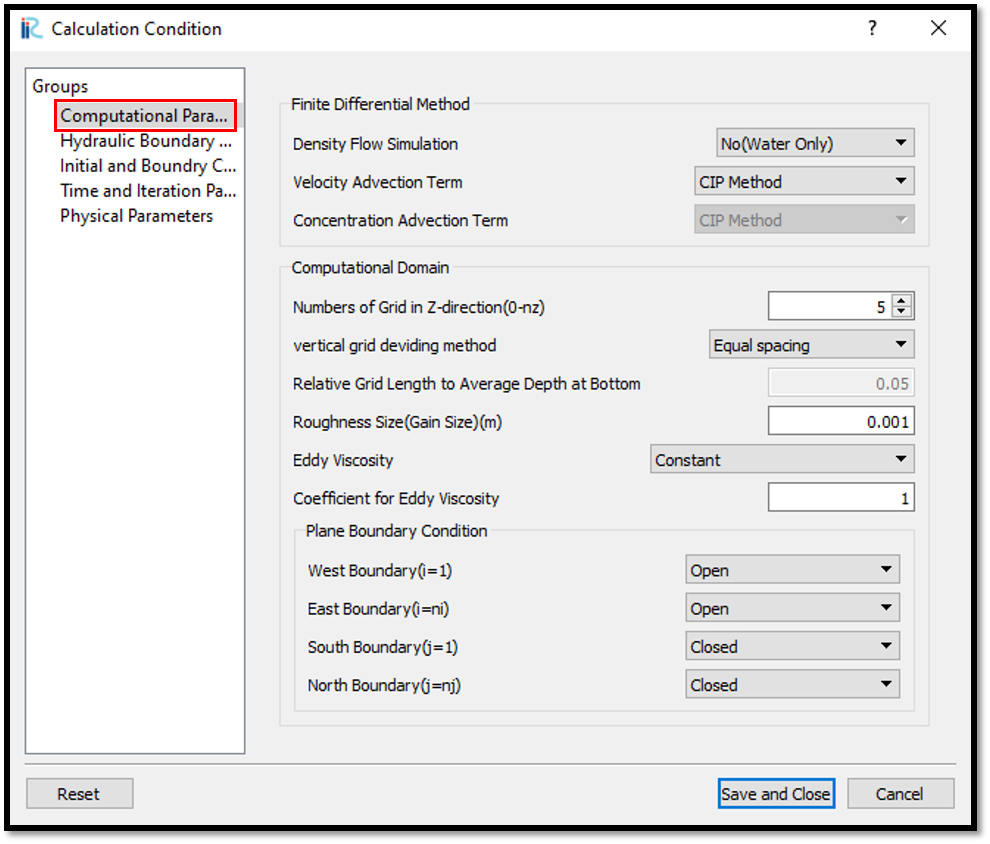
Figure 137 : Calculation Condition : Computational Parameters

Then give hydraulic boundary conditions. Since the boundary conditions are open boundaries , boundary condition needs to be given as shown in Figure 138.

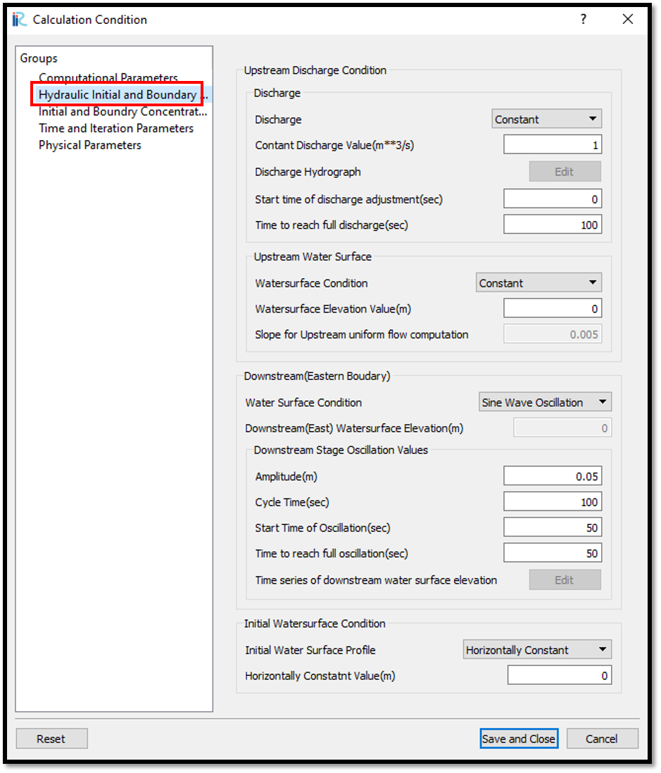
Figure 138 : Calculation Condition : Boundary Conditions

Then give initial and Boundary concentrations as shown in Figure 139. Here only water is used for simulation, initial and boundary concentartion window is inactive.

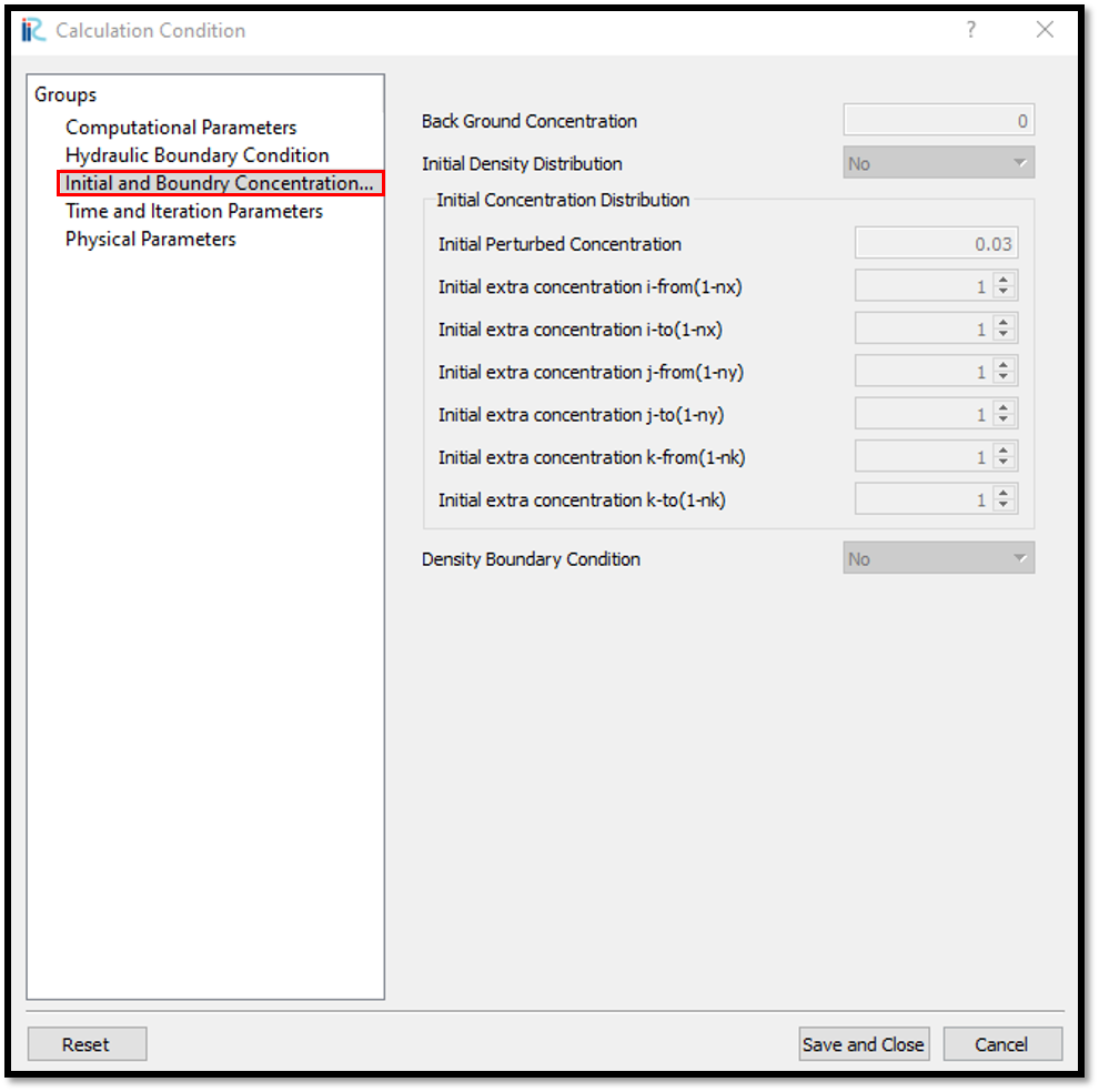
Figure 139 : Calculation Condition : Initial and Boundary Concentrations

Then the time and iteration parameters are give as shown in Figure 140.

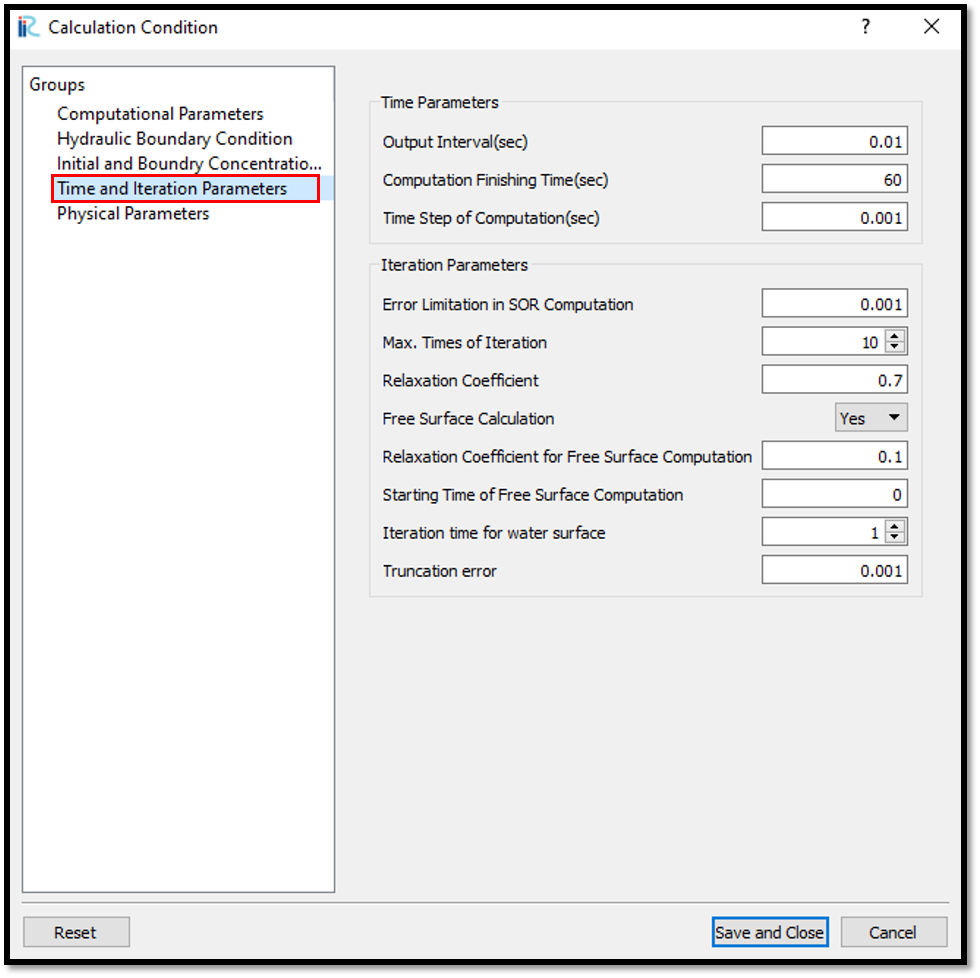
Figure 140 : Calculation Condition : Time and Iteration parameters

Then give the physical parameters as given in Figure 141.

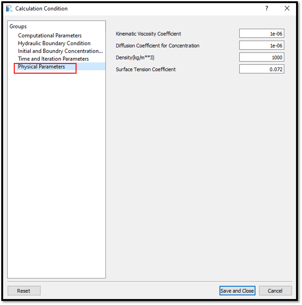
Figure 141 : Calculation Condition : Physical Parameters

After setting the calculation conditions, save the project by clicking on save tab. Now start simulation by, [Simulation] [Run]. Simulation will start and after some time it will finish showing the message the solver finished the calculation.

Visualization of results

Open 3D post processing window by selecting, [Calculation Results] [Open new 3D Post-Processing Window].

In this example, linear plots will be demonstrated. For linear graphs, click on linear graph icon in top of the window as shown in Figure 142. Or else go to [Calculation Results] - [Open new graph window]. Then the data source setting window will appear as shown in figure.

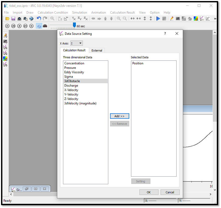
Figure 142 : Visualization of Results : Data sorce setting window

Here x axis and the 3dimensional data need be selected. Here Position vs Distance is selceted to plot. Therefore, axis is set i and position is selected for 3dimensional data. The resulting plot is as shown in Figure 143.

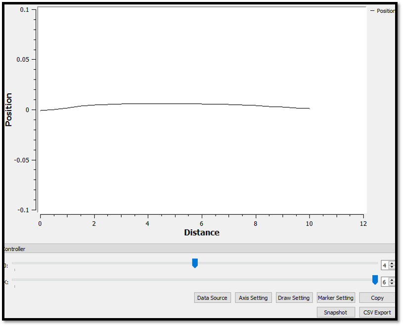
Figure 143 : Visualization of Results : Position vs Distane plot

If we need to plot position vs time, data source setting has to be done as shown in Figure 144.

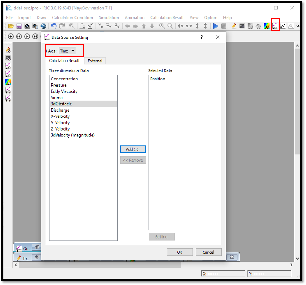
Figure 144 : Visualization of Results : Data source setting

The resulting plot can be seen as shown in Figure 145.

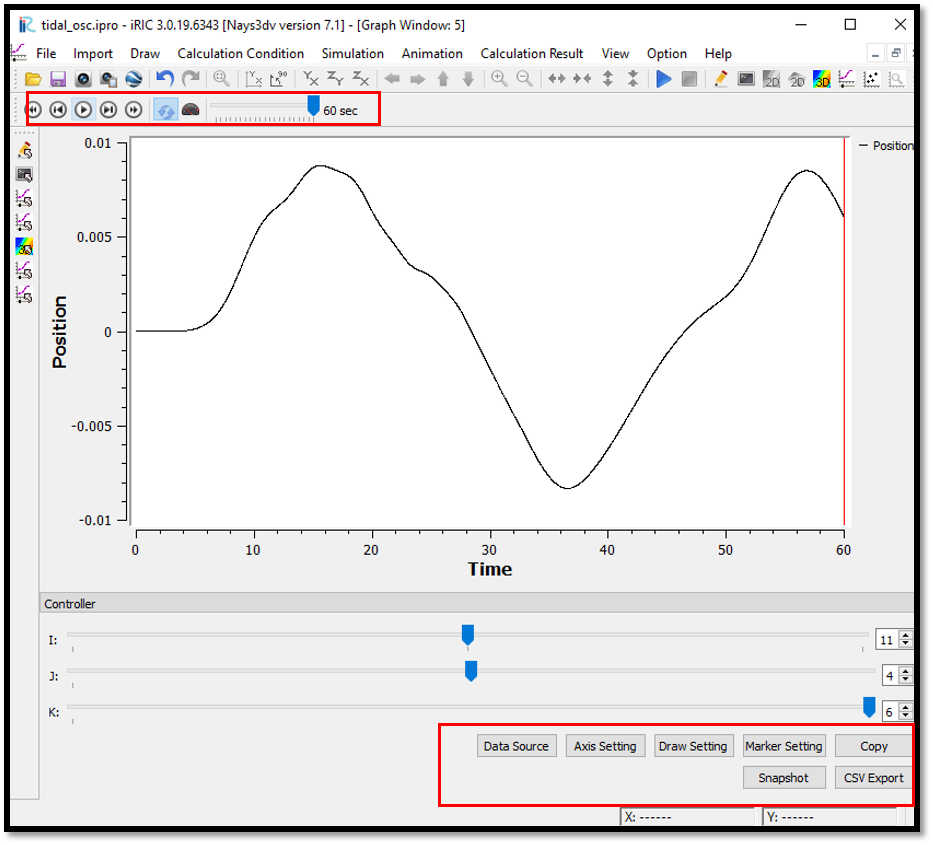
Figure 145 : Visualization of Results : Position vs Time plot

As shown in the down of the graphs there are several options available for line graphs such as export csv format, copy, axis setting etc.